GCJ – Cookie Clicker Alpha

Cookie Clicker Alpha, Qualification Round 2014.

This problem is also fairly simple, and we can solve it with a straightforward algorithm. Many thanks to both Dashamir and Karell who pointed out ways to simplify my original solution in the comments.

We want to decide for each farm if we’ll be able to win faster without buying the next farm (which will take time) or with buying the next farm (which will take time to save up cookies to buy the farm and a further time to win with the new, higher, production rate. If we don’t buy the farm, we report the current time plus the time to win with the current rate. If we do buy the farm, then we just repeat the step above after incrementing our rate and time to account for the new farm purchase.

def solve_case(case):
    C, F, X = case
    
    rate = 2.0
    time = 0.0

    while True:
        time_if_wait = X / rate
        time_if_buy = C / rate + X / (rate + F)
        if time_if_wait <= time_if_buy:
            return time + time_if_wait
        time += C / rate
        rate += F

GCJ – Magic Trick

Magic Trick, Qualification Round 2014.

Just as a reminder, all the Google Code Jam code and solutions I’m posting are based off of the template code I posted last year. It handles all the homework of reading and writing files properly and allows me to simply focus on solving the problem. I’ll generally only post the solve_case function and leave the rest to you.

As the first problem in the Qualification Round, this problem is more a test of basic coding ability than algorithm design. We’re given two 4 by 4 arrays and a row is chosen from each of them. The number of interest is supposed to be found in each of the chosen rows of the two arrays. So we want to find all numbers that are in both rows. We can do this quite easily using Python sets, although be careful of the indexing change from the row numbers we’re given (1 to 4) and the way Python indexes arrays (0 to 3). Once we have our list of potential numbers, then if there’s exactly one, that must be the one we want. If there’s more than two, the magician didn’t choose the arrays properly, and if there’s none, then the volunteer must be cheating.

def solve_case(case):
    ans1, grid1, ans2, grid2 = case
    
    valid = set(grid1[ans1-1]) & set(grid2[ans2-1])
    
    if len(valid) == 1:
        return valid.pop()
    elif len(valid) > 1:
        return "Bad magician!"
    else:
        return "Volunteer cheated!"

GCJ – Minesweeper Master

Minesweeper Master, Qualification Round 2014

There are a couple of key insights necessary to solve this problem. We know how many mines there will be and the size of the board, and we want to find some board state that would clear all the empty squares at once. It doesn’t have to be a likely state, it just has to be a valid state given the board size and mine count. So we can rearrange the board at will to find a state that will work.

The first insight is that for the board to clear in one click, all the empty spaces must be contiguous. Because a square can’t cascade to a square it’s not next to, we have to bunch all the empty squares together in one region.

The second insight is that this empty region should be up against the corner. Suppose we have a 2 by 2 clear area in a 4 by 4 region with mines surrounding it. If the empty region is in the middle or on the side, like this,

**** ****
*..* ****
*..* *..*
**** *..*

then all of the empty squares are next to a mine and they won’t cascade. If the empty region is in the corner,

****
****
..**
..**

then the corner square is next to the edge of the board rather than mines and will cascade, and we can win in a single click. So not only should our empty region be in the corner, but the clicked square should always be the corner square. Other squares might be able to cascade, but the corner one definitely will if others could.

With these insights, it’s now a matter of figuring out how to build our empty region and how to tell if it will cascade properly.

To build it, first note that if we can fill up a whole row or whole column of the board with mines, then we should do so. We’ll start up with the empty region filling the whole board, fill the shortest whole row or whole column available with mines, and repeat until we don’t have enough mines to keep going. At that point, we’ll have an empty rectangular region with the clicked square in the corner and some uneven number of mines to keep placing. If we have no mines, then we’ve finished our board and found a good position. We just need to check and make sure that the corner will cascade. If it won’t, then the board position doesn’t work with a single click and won’t be possible.

If we do still have mines to place, we’ll start placing them along the sides kitty corner to the clicked corner, like so:

c..**
...**
..***
*****

But we’re limited in how many we can place, because the rest of those rows and columns have to be cleared as well. We have to leave at least two empty squares at the edge of both the row and the column. With only a single empty square, the empty square next to it won’t cascade and we won’t clear the singleton:

c..**
..***
..***
*****

So the most we can place is the length of the empty space plus the width of the empty space minus five – two for the row, two for the column, and one for the overlap. If the number of mines to place is less than this, then we do so and report the board position. If not, then it’s impossible. That, along with some careful outlining of edge cases, will solve the problem.

def solve_case(case):
    R, C, M = case
    free = R * C - M
    
    def write_board(board):
        d = {0:'.', 1:'c', 2:'*'}
        return '\n' + '\n'.join([''.join([d[n] for n in r])for r in board]) + '\n'
    
    board = np.zeros((R, C), dtype=int)
    board[0,0] = 1
    
    while min(R, C) <= M:
        if R < C:
            board[:,C-1] = 2
            C -= 1
            M -= R
        elif C <= R:
            board[R-1,:] = 2
            R -= 1
            M -= C
    
    def cascades(board, r, c):
        rows = [i for i in (r-1, r, r+1) if (i >= 0 and i < board.shape[0])]
        cols = [i for i in (c-1, c, c+1) if (i >= 0 and i < board.shape[1])]
        for r in rows:
            for c in cols:
                if board[r,c] == 2:
                    return False
        return True
    
    if M == 0:
        if cascades(board, 0, 0) or free == 1:
            return write_board(board)
        else:
            return "\nImpossible"
    
    if M > (R + C - 5):
        return "\nImpossible"
        
    if R <= 2 or C <= 2:
        return "\nImpossible"
        
    fill_num = min(M, R - 2)
    board[(R - fill_num):,C-1] = 2
    M -= fill_num
    
    fill_num = min(M, C - 3)
    board[R-1,(C - fill_num - 1):] = 2
    M -= fill_num
    
    return write_board(board)

GCJ – Deceitful War

Deceitful War, Qualification Round 2014.

This was a fun one. There are three strategies that we need to figure out and take into account when we’re writing our solution:

1. Ken’s optimal strategy for playing normal War.
2. Naomi’s optimal strategy for playing normal War.
3. Naomi’s optimal strategy for playing Deceitful War.

Let’s start with Ken’s strategy. As far as he knows, Naomi accurately tells him the weight of the block she has chosen, and then he gets to pick one of his blocks to play. Which block should he pick? Well, he always wants to win. So if he can, he should pick a block of his that is larger than . Of those blocks that are larger, he should use the smallest, because that will allow the larger blocks to be used later and potentially win more rounds. If he has no blocks larger than , then he should just use the smallest block he has. He can’t win this round, so he may as well avoid wasting any of his heavier blocks.

When Naomi plays normal War, she gets to pick the order in which she plays her blocks. Which block should she pick? We know that if she picks a block which Ken can beat, he’ll play the smallest block that can beat it. Otherwise, he’ll play his smallest block. She wants to force Ken to play his highest blocks, and the best way to do that is to play her highest blocks. So she’ll play her blocks in order from largest to smallest, giving her the best possible score without knowing the weights of Ken’s blocks.

But when Naomi plays Deceitful War she not only gets to choose the order of her blocks, she also gets to lie to Ken about the weight of her blocks. She can’t lie to win matches that she otherwise would have lost, because then Ken will figure out that she’s cheating. But she can lie to force Ken to use different, larger, blocks than he otherwise would have. Start with Naomi’s smallest block. If it’s smaller than Ken’s smallest block, then she can’t possibly win with it. But she can lie about its weight and force Ken to use his largest block to beat it, by telling Ken its weight is between his largest and his second-largest block. If it’s larger than Ken’s smallest block, then she can win by lying about its weight, telling Ken it’s bigger than his biggest block. Ken will then play his smallest block, and Naomi will win. Naomi can keep going through her blocks like this from smallest to largest, systematically lying and get the most wins possible without Ken finding out about her deceit.

def ken_choice(told_naomi, ken):
    for j in range(len(ken)):
        if ken[j] > told_naomi:
            return ken.pop(j)
    return ken.pop(0)

def normal_war(naomi, ken):
    score = 0
    for i in range(len(naomi))[::-1]:
        if naomi[i] > ken_choice(naomi[i], ken):
            score += 1
    return score

def deceitful_war(naomi, ken):
    score = 0
    for i in range(len(naomi)):
        if naomi[0] > ken[0]:
            score += 1
            ken.pop(0)
        else:
            ken.pop(-1)
        naomi.pop(0)
    return score

def solve_case(case):
    naomi, ken = case
    naomi.sort()
    ken.sort()
    normal = normal_war(naomi.tolist(), ken.tolist())
    deceitful = deceitful_war(naomi.tolist(), ken.tolist())
    return "%i %i" % (deceitful, normal)

GCJ – Garbled Email

Garbled Email, Round 1B 2013.

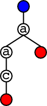
This is a tricky problem.  The first tricky part is figuring out an efficient way to store the dictionary so that we can quickly identify whether a particular substring is a prefix of a word in the dictionary.  This is a well-studied problem, and the right data structure is a trie.  Suppose we’re working with a small dictionary containing the words a, aac, acb, baa, bbc, bc, caba, caab.  We’ll start our trie with an empty node, and then keep adding words until we’re finished.  We start by adding the word a.  We link a node with the letter a to the root, and then link a marker node to that to show that this is the end of a word.

Next, we’ll add in the word aac. We already have the letter a linked to the root, so we go there and add more letters to that node.

And we repeat this until all the words are in the tree. For each letter in the new word, if that letter is already a child of the current node, we walk to that child. If not, we create a new child. Once we’re at the end of the word, we add a marker child to the last node denoting the end of the word. After we’re finished with our small dictionary, we end up with this:

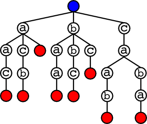
Each of the red nodes marks the end of a word, so we can see that we have all eight words in the trie.

Now that we have our data stored in an easily-accessible manner, let’s start with a simpler problem than the one asked.  Suppose that there was no garbling, just spaces removed, and we’re given some string, say, aacaabbc.  How can we use this structure to quickly find out whether this string could be divided up into words from our dictionary?  Start at the root of the tree and look at the first letter a of the string.  a is a child of our current node, so we’ll walk to that node and move to the next letter.  Here we see an end node as a child, marking that we’ve now finished a possible node.  So we know we can split off the word a from our string, leaving acaabbc behind.  This split will produce a valid word separation for the whole string if and only if acaabbc can itself be divided up into words from our dictionary.

First, though, we need to finish walking down and make sure we’ve found the only possible split.  The next letter is a, which is a child of our current node, so we move there.  This node has no end node as a child, so it’s not a possible word separation.  The third letter is c, which is a child of this node, so we’ll move there next.  This node is another word separation, giving us aac as the first word and aabbc as the remainder of the string.  There are no other children of this node, so these are the only possible word separations.

So we now know that aacaabbc is divisible into words if and only if at least one of its two suffixes acaabbc and aabbc are divisible into words.  This suggests that we might be able to use dynamic programming for our problem.  We can create an array of boolean variables telling us whether each suffix of our string can be divided into words.  We can look at the suffixes of our string in order of increasing size and calculate whether each of them is divisible.  The larger suffixes can then use the calculations previously done on the smaller suffixes to quickly calculate whether they themselves are divisible.

Starting with the smallest suffix, c, we quickly find that it is not a word, so we mark that index as False.  bc, the next smallest, so we mark it as True, and similarly for bbc.  abbc gives a potential split at a|bbc, and we know that bbc is True, so abbc must be True as well.  We then keep working backwards until we reach the beginning of the string, and then the final answer is simply the result in the first element of our array.  Doing this we quickly find that aacaabba is in fact divisible.

So this works for messages where there is no garbling at all.  Now let’s add the garbling in and see if we can work out a solution.  We’ll simplify the problem slightly, though, by allowing any character in the string to be garbled, ignoring the constraints on how close the garbled characters are allowed to be.  Suppose we have the string abbbcbba.  We can work backwards, just as before, from smaller to larger suffixes.  This time, though, instead of only storing whether or not a suffix is divisible into words, we’ll store how many changes are needed to make it divisible.

c alone, for instance, isn’t a word, but we can change it into a with a single substitution, so our answer is one.  The next two suffixes, bc and bbc, are both words, so they get values of zero.  cbbc isn’t valid, but if we swap it to abbc we can split it at a|bbc, giving us two valid words, for an answer of one.  We keep working backwards just as before, looking for all possible words we can construct at the start of our suffix, splitting it, and then putting the minimum changes required into our array.  Once we’re finished, the final answer is just the result in the first element of our array.  So we find that abbbcbbc can be made divisible with only a single character swap.

Finally, we want to incorporate the closeness requirements for our garbled characters – changes must have at least four non-garbled characters between them.  Now for each suffix we want to store five different values, giving the minimum changes required for this suffix when the first x characters are required to match perfectly, with x ranging between 0 and 4 inclusive.  Let’s look at this array for the string abbbcbba.

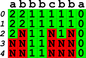
Here N is marking divisions that are not possible at all.  Otherwise, we fill the array with the number of changes required.  Again, let’s start at the back and move towards the front of the string.  a, the last suffix, is a word itself, so we fill its column with zeros.  ba is not a word, but could be divisible if we change one of the characters, to either bc or a|a.  The bottom three rows require us to keep the first two characters unchanged, so those entries are marked as N.  Both of the top two are possible with only a single change.  bba is valid only if changed into bbc, which requires no more than two characters held unchanged, so we mark up the column appropriately.  We continue in the same manner, looking for potential word divisions and marking down the minimum changes required that allow the required distance between changes.  Then, just as with the simpler problems, we read off our final answer as the entry in the first column and the first row.  

GCJ – Consonants

Consonants – Round 1C 2013

The first thing to notice about this problem is that in order to identify substrings containing at least n consonants we will need to identify any stretches of exactly n consonants in the word.  Obviously, if there are no such stretches in the word, then there are no possible substrings containing n consecutive consonants.

Suppose instead we find exactly one such substring, as with the sample word quartz with an n-value of 3.

A simple sample word.

The only valid stretch here is from index 3 to 5. How many total substrings can be made that contain this stretch of consonants? Well, we can vary the start of the substring from 0 to 3 and the end of the substring from 5 to 5, and both the start and the end of the substring can be varied independently, which gives us total possible substrings containing this stretch.

We can then generalize this to an arbitrary word of length L, containing only a single stretch of n consecutive consonants.  The stretch begins at index i and ends at index j, where . Then there are possible positions for the start of substrings containing this stretch (all indices from 0 to i inclusive) and possible positions for the end of substrings containing this stretch (all indices from j to L – 1 inclusive). Since these choices of start and end positions are independent, that gives us possible substrings.

Now we need to expand our analysis to words containing multiple stretches of consonants.

A slightly more complex sample word.

In the word straight we have two disjoint consonant stretches of length n=3, [0, 2] and [5, 7]. Moving from left to right, we can start by applying our previous analysis to the first substring, giving us 6 possible substrings containing the stretch [0, 2]. Applying the same calculation to the second stretch, we calculate 6 substrings containing it. So we can add these and get a total of 12, right? Well, no, as you can see from the problem statement the correct answer is 11, because we double-counted the substring [0, 7], which contains both stretches of consonants.

So for stretches after the first, we want to calculate not the number of substrings containing it, but the number of substrings that both contain it and do not contain any previously analyzed substrings. Since we’re analyzing substrings from left to right, we can do this by running the left index of the substring not from 0 to i but instead from k + 1 to i, where k is the start index of the previous substring. That gives us new substrings containing this stretch of consonants. If we do this with i, j, k = 5, 7, 0 for the second substring, we get 5, which gives us the correct answer when added to the 6 substrings containing the first substring.

A sample word with overlapping stretches of consonants.

Now we want to check and make sure that we get the correct answer for words with overlapping stretches of n consonants. The word gcj contains two such stretches, [0, 1] and [1, 2]. With our methods, we obtain 2 substrings containing the first and 1 containing the second but not the first, which is the correct answer.

Finally, we need to quickly identify all such stretches in the word from left to right. We can do this by iterating through each letter in a word. If this letter is a consonant, we increment the size of the current stretch of consonants, while capping the size at n. If it is not a consonant, we set the size to 0. Then, if the size is n, we are located at the end of a stretch of n consonants, and we should increment our count of substrings by .

However, we are only keeping track of the current position, which is at the end of the active stretch of consonants, or k, so we need to calculate i in terms of k, which is simply . We then substitute this into our last expression, giving the number of additional substrings contributed by each stretch of consonants as .

GCJ – Falling Diamonds

Falling Diamonds, Round 1B 2013

GCJ – Osmos

Osmos, Round 1B 2013

This was a fun little problem in recursion. We have a mote that wants to eat other smaller motes, and we want to enable our mote to eat all of the others by either removing uneatable motes or adding new, eatable ones. The first thing to notice is that given a set of motes to try to eat, it is always optimal to try to eat the smallest mote. If we can’t eat it, then we know that we also can’t eat any of the larger motes, and if we can eat it, then we’ll only be larger afterwards, able to eat at least as many of the remaining motes as we could before. Secondly, if we want to remove uneatable motes, it’s always optimal to remove the largest motes we can.  If there are any uneatable motes, then the largest must be one of them, and removing it won’t impede our ability to eat any larger motes, if we decide to add more motes later. Thirdly, if we do wish to add a mote to enable our mote to eat others, it is optimal to always add the largest mote that we can currently eat, which will be 1 unit smaller than our current size.

Together, these suggest that the first thing we want to do is sort the motes from smallest to largest and analyze them in order.  For each mote, we have two possibilities:  first, it may be small enough to eat, in which case we eat it, our mote gets larger, and we move on to the next smallest mote.  Second, it may be too big to eat, in which case we can either add another mote just smaller than our current size in hopes that eating it will allow our mote to grow large enough to continue, or we can simply remove all the remaining motes and be finished.  Which of these we choose depends on which will cost fewer changes.  Removing all remaining motes will cost L, where L is the number of motes remaining.  Adding an additional mote will cost 1 plus the number of changes it takes to eat the remaining motes with our new larger mote.

In general, the cost of eating a list of motes with a mote of size is

We can calculate this fairly simply with a recursive formula. Our base cases will be , where A can never grow and we must remove all motes and , where there are no motes remaining, and we simply return 0. For other cases, if we can eat the first mote, then we recursively call with incremented by and removed from . If we cannot, then we return the minimum of , and the recursive call with incremented by .

Of note is that this can lead to a recursive stack as large as , but as this is limited to 100 in the problem statement, we shouldn’t have to worry about space limitations with this solution.

GCJ – Manage Your Energy

Manage Your Energy, Round 1A 2013

GCJ – Bullseye

Bullseye, Round 1A 2013

This is a largely mathematical problem: the first ring will use  units of paint, the second  units, and so forth, so that the  ring will require
, or

units of paint. I.e., each ring will take a constant amount of paint () plus some varying amount depending on how far out it is (). That second sequence is 1, 5, 9, 13, 17, 21, etc. But the question we want to answer is not how much paint each ring will take, but how many rings we can paint with a given amount of paint.

One way to solve this problem would be to simply add up the paint as we paint each ring until we don’t have enough paint to go on, then report the number of the last complete ring. This solution will work for the small problem, but will fail on the large problem as it is linear in , and in the large problem can be very very large.

We can resolve this by finding a closed form solution for the sum of all from 1 to k. We first note that there is a constant amount of paint for each ring, so we can sum up that part simply as . The first few variable sums are 1, 6, 15, 28, 45…, which we can recognize as the sequence of hexagonal numbers with closed form solution . This gives us:

Now that we have a closed form solution, we can try to substitute in , the total amount of paint we have, for , solve for , and round down to obtain the maximum number of complete rings we can draw, in constant time, much better than linear! This is a quadratic, and we obtain the (positive) solution

We’re done, right? Well, this solution will work fine for the small input, and in constant time. But it will fail dramatically on the large input. Why? Because we’re taking square roots of very large integers, which transforms them from integers (which are stored with perfect precision) to floating point numbers (which are stored with limited precision), and with the limits we’re given, the precision of floating points isn’t sufficient to give us the right answer this way.

So we need to use a different method. Again, what we want to do is find such that while . Simply walking through increasing values of is too slow for the large input. So instead we can do a binary search. We’re guaranteed in the problem statement that . So let’s start a lower limit for our search at . We’ll start an upper limit at . It’s probably not an upper limit yet, but we’ll make it so by iteratively doubling both our limits until it is: find the first power of 2 where . Then is somewhere in the interval . We can find its exact value by repeatedly subdividing this interval until it is narrowed down to a single value.